Determine the fundamental system of solutions for a homogeneous slough. How to find a nontrivial and fundamental solution to a system of linear homogeneous equations
Solving systems of linear algebraic equations (SLAEs) is undoubtedly the most important topic in a linear algebra course. A huge number of problems from all branches of mathematics come down to solving systems linear equations. These factors explain the reason for this article. The material of the article is selected and structured so that with its help you can
- choose the optimal method for solving your system of linear algebraic equations,
- study the theory of the chosen method,
- solve your system of linear equations by considering detailed solutions to typical examples and problems.
Brief description of the article material.
First, we give all the necessary definitions, concepts and introduce notations.
Next, we will consider methods for solving systems of linear algebraic equations in which the number of equations is equal to the number of unknown variables and which have a unique solution. Firstly, we will focus on Cramer’s method, secondly, we will show the matrix method for solving such systems of equations, and thirdly, we will analyze the Gauss method (the method of sequential elimination of unknown variables). To consolidate the theory, we will definitely solve several SLAEs in different ways.
After this, we will move on to solving systems of linear algebraic equations of general form, in which the number of equations does not coincide with the number of unknown variables or the main matrix of the system is singular. Let us formulate the Kronecker-Capelli theorem, which allows us to establish the compatibility of SLAEs. Let us analyze the solution of systems (if they are compatible) using the concept of a basis minor of a matrix. We will also consider the Gauss method and describe in detail the solutions to the examples.
We will definitely dwell on the structure of the general solution of homogeneous and inhomogeneous systems of linear algebraic equations. Let us give the concept of a fundamental system of solutions and show how the general solution of a SLAE is written using the vectors of the fundamental system of solutions. For a better understanding, let's look at a few examples.
In conclusion, we will consider systems of equations that can be reduced to linear ones, as well as various problems in the solution of which SLAEs arise.
Page navigation.
Definitions, concepts, designations.
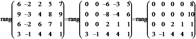
We will consider systems of p linear algebraic equations with n unknown variables (p can be equal to n) of the form
Unknown variables, - coefficients (some real or complex numbers), - free terms (also real or complex numbers).
This form of recording SLAE is called coordinate.
IN matrix form writing this system of equations has the form,
Where  - the main matrix of the system, - a column matrix of unknown variables, - a column matrix of free terms.
If we add a matrix-column of free terms to matrix A as the (n+1)th column, we get the so-called extended matrix systems of linear equations. Typically, an extended matrix is denoted by the letter T, and the column of free terms is separated by a vertical line from the remaining columns, that is, 
Solving a system of linear algebraic equations called a set of values of unknown variables that turns all equations of the system into identities. The matrix equation for given values of the unknown variables also becomes an identity.
If a system of equations has at least one solution, then it is called joint.
If a system of equations has no solutions, then it is called non-joint.
If a SLAE has a unique solution, then it is called certain; if there is more than one solution, then – uncertain.
If the free terms of all equations of the system are equal to zero ![]() , then the system is called homogeneous, otherwise - heterogeneous.
, then the system is called homogeneous, otherwise - heterogeneous.
Solving elementary systems of linear algebraic equations.
If the number of equations of a system is equal to the number of unknown variables and the determinant of its main matrix is not equal to zero, then such SLAEs will be called elementary. Such systems of equations have a unique solution, and in the case of a homogeneous system, all unknown variables are equal to zero.
We began to study such SLAEs in high school. When solving them, we took one equation, expressed one unknown variable in terms of others and substituted it into the remaining equations, then took the next equation, expressed the next unknown variable and substituted it into other equations, and so on. Or they used the addition method, that is, they added two or more equations to eliminate some unknown variables. We will not dwell on these methods in detail, since they are essentially modifications of the Gauss method.
The main methods for solving elementary systems of linear equations are the Cramer method, the matrix method and the Gauss method. Let's sort them out.
Solving systems of linear equations using Cramer's method.
Suppose we need to solve a system of linear algebraic equations 
in which the number of equations is equal to the number of unknown variables and the determinant of the main matrix of the system is different from zero, that is, .
Let be the determinant of the main matrix of the system, and ![]() - determinants of matrices that are obtained from A by replacement 1st, 2nd, …, nth column respectively to the column of free members:
- determinants of matrices that are obtained from A by replacement 1st, 2nd, …, nth column respectively to the column of free members: 
With this notation, unknown variables are calculated using the formulas of Cramer’s method as  . This is how the solution to a system of linear algebraic equations is found using Cramer's method.
Example.
Cramer's method  .
.
Solution.
The main matrix of the system has the form  . Let's calculate its determinant (if necessary, see the article):
Since the determinant of the main matrix of the system is nonzero, the system has a unique solution that can be found by Cramer’s method.
Let's compose and calculate the necessary determinants ![]() (we obtain the determinant by replacing the first column in matrix A with a column of free terms, the determinant by replacing the second column with a column of free terms, and by replacing the third column of matrix A with a column of free terms):
(we obtain the determinant by replacing the first column in matrix A with a column of free terms, the determinant by replacing the second column with a column of free terms, and by replacing the third column of matrix A with a column of free terms): 
Finding unknown variables using formulas  :
:
Answer:
The main disadvantage of Cramer's method (if it can be called a disadvantage) is the complexity of calculating determinants when the number of equations in the system is more than three.
Solving systems of linear algebraic equations using the matrix method (using an inverse matrix).
Let a system of linear algebraic equations be given in matrix form, where the matrix A has dimension n by n and its determinant is nonzero.
Since , matrix A is invertible, that is, there is an inverse matrix. If we multiply both sides of the equality by the left, we get a formula for finding a matrix-column of unknown variables. This is how we obtained a solution to a system of linear algebraic equations using the matrix method.
Example.
Solve system of linear equations matrix method.
Solution.
Let's rewrite the system of equations in matrix form: 
Because
then the SLAE can be solved using the matrix method. By using inverse matrix the solution to this system can be found as  .
.
Let's construct an inverse matrix using a matrix from algebraic additions of elements of matrix A (if necessary, see the article): 
It remains to calculate the matrix of unknown variables by multiplying the inverse matrix  to a matrix-column of free members (if necessary, see the article):
Answer:
 or in another notation x 1 = 4, x 2 = 0, x 3 = -1.
The main problem when finding solutions to systems of linear algebraic equations using the matrix method is the complexity of finding the inverse matrix, especially for square matrices of order higher than third.
Solving systems of linear equations using the Gauss method.
Suppose we need to find a solution to a system of n linear equations with n unknown variables 
the determinant of the main matrix of which is different from zero.
The essence of the Gauss method consists of sequentially eliminating unknown variables: first, x 1 is excluded from all equations of the system, starting from the second, then x 2 is excluded from all equations, starting from the third, and so on, until only the unknown variable x n remains in the last equation. This process of transforming system equations to sequentially eliminate unknown variables is called direct Gaussian method. After completing the forward stroke of the Gaussian method, x n is found from the last equation, using this value from the penultimate equation, x n-1 is calculated, and so on, x 1 is found from the first equation. The process of calculating unknown variables when moving from the last equation of the system to the first is called inverse of the Gaussian method.
Let us briefly describe the algorithm for eliminating unknown variables.
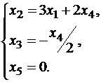
We will assume that , since we can always achieve this by rearranging the equations of the system. Let's eliminate the unknown variable x 1 from all equations of the system, starting with the second. To do this, to the second equation of the system we add the first, multiplied by , to the third equation we add the first, multiplied by , and so on, to the nth equation we add the first, multiplied by . The system of equations after such transformations will take the form 
where and  .
.
We would have arrived at the same result if we had expressed x 1 in terms of other unknown variables in the first equation of the system and substituted the resulting expression into all other equations. Thus, the variable x 1 is excluded from all equations, starting from the second.
Next, we proceed in a similar way, but only with part of the resulting system, which is marked in the figure 
To do this, to the third equation of the system we add the second, multiplied by , to fourth equation let's add the second multiplied by , and so on, to the nth equation we add the second multiplied by . The system of equations after such transformations will take the form 
where and  . Thus, the variable x 2 is excluded from all equations, starting from the third.
Next, we proceed to eliminating the unknown x 3, while we act similarly with the part of the system marked in the figure 
So we continue the direct progression of the Gaussian method until the system takes the form 
From this moment we begin the reverse of the Gaussian method: we calculate x n from the last equation as , using the obtained value of x n we find x n-1 from the penultimate equation, and so on, we find x 1 from the first equation.
Example.
Solve system of linear equations Gauss method.
Solution.
Let us exclude the unknown variable x 1 from the second and third equations of the system. To do this, to both sides of the second and third equations we add the corresponding parts of the first equation, multiplied by and by, respectively: 
Now we eliminate x 2 from the third equation by adding to its left and right sides the left and right sides of the second equation, multiplied by: 
This completes the forward stroke of the Gauss method; we begin the reverse stroke.
From the last equation of the resulting system of equations we find x 3: 
From the second equation we get .
From the first equation we find the remaining unknown variable and thereby complete the reverse of the Gauss method.
Answer:
X 1 = 4, x 2 = 0, x 3 = -1.
Solving systems of linear algebraic equations of general form.
In general, the number of equations of the system p does not coincide with the number of unknown variables n:
Such SLAEs may have no solutions, have a single solution, or have infinitely many solutions. This statement also applies to systems of equations whose main matrix is square and singular.
Kronecker–Capelli theorem.
Before finding a solution to a system of linear equations, it is necessary to establish its compatibility. The answer to the question when SLAE is compatible and when it is inconsistent is given by Kronecker–Capelli theorem:
In order for a system of p equations with n unknowns (p can be equal to n) to be consistent, it is necessary and sufficient that the rank of the main matrix of the system be equal to the rank of the extended matrix, that is, Rank(A)=Rank(T).
Let us consider, as an example, the application of the Kronecker–Capelli theorem to determine the compatibility of a system of linear equations.
Example.
Find out whether the system of linear equations has  solutions.
Solution.
 . Let's use the method of bordering minors. Minor of the second order
  different from zero. Let's look at the third-order minors bordering it:
Since all the bordering minors of the third order are equal to zero, the rank of the main matrix is equal to two.
In turn, the rank of the extended matrix  is equal to three, since the minor is of third order
different from zero.
Thus, Rang(A), therefore, using the Kronecker–Capelli theorem, we can conclude that the original system of linear equations is inconsistent.
Answer:
The system has no solutions.
So, we have learned to establish the inconsistency of a system using the Kronecker–Capelli theorem.
But how to find a solution to an SLAE if its compatibility is established?
To do this, we need the concept of a basis minor of a matrix and a theorem about the rank of a matrix.
The minor of the highest order of the matrix A, different from zero, is called basic.
From the definition of a basis minor it follows that its order is equal to the rank of the matrix. For a non-zero matrix A there can be several basis minors; there is always one basis minor.
For example, consider the matrix  .
.
All third-order minors of this matrix are equal to zero, since the elements of the third row of this matrix are the sum of the corresponding elements of the first and second rows.
The following second-order minors are basic, since they are non-zero 
Minors  are not basic, since they are equal to zero.
Matrix rank theorem.
If the rank of a matrix of order p by n is equal to r, then all row (and column) elements of the matrix that do not form the chosen basis minor are linearly expressed in terms of the corresponding row (and column) elements forming the basis minor.
What does the matrix rank theorem tell us?
If, according to the Kronecker–Capelli theorem, we have established the compatibility of the system, then we choose any basis minor of the main matrix of the system (its order is equal to r), and exclude from the system all equations that do not form the selected basis minor. The SLAE obtained in this way will be equivalent to the original one, since the discarded equations are still redundant (according to the matrix rank theorem, they are a linear combination of the remaining equations).
As a result, after discarding unnecessary equations of the system, two cases are possible.
If the number of equations r in the resulting system is equal to the number of unknown variables, then it will be definite and the only solution can be found by the Cramer method, the matrix method or the Gauss method.
Example.
 .
.
Solution.
Rank of the main matrix of the system  is equal to two, since the minor is of second order
  different from zero. Extended Matrix Rank
  is also equal to two, since the only third order minor is zero
and the second-order minor considered above is different from zero. Based on the Kronecker–Capelli theorem, we can assert the compatibility of the original system of linear equations, since Rank(A)=Rank(T)=2.
As a basis minor we take . It is formed by the coefficients of the first and second equations: 
The third equation of the system does not participate in the formation of the basis minor, so we exclude it from the system based on the theorem on the rank of the matrix: 
This is how we obtained an elementary system of linear algebraic equations. Let's solve it using Cramer's method: 
Answer:
x 1 = 1, x 2 = 2.
If the number of equations r in the resulting SLAE less number unknown variables n, then on the left sides of the equations we leave the terms that form the basis minor, and we transfer the remaining terms to the right sides of the equations of the system with the opposite sign.
The unknown variables (r of them) remaining on the left sides of the equations are called main.
Unknown variables (there are n - r pieces) that are on the right sides are called free.
Now we believe that free unknown variables can take arbitrary values, while the r main unknown variables will be expressed through free unknown variables in a unique way. Their expression can be found by solving the resulting SLAE using the Cramer method, the matrix method, or the Gauss method.
Let's look at it with an example.
Example.
Solve a system of linear algebraic equations  .
.
Solution.
Let's find the rank of the main matrix of the system  by the method of bordering minors. Let's take a 1 1 = 1 as a non-zero minor of the first order. Let's start searching for a non-zero minor of the second order bordering this minor:
This is how we found a non-zero minor of the second order. Let's start searching for a non-zero bordering minor of the third order: 
Thus, the rank of the main matrix is three. The rank of the extended matrix is also equal to three, that is, the system is consistent.
We take the found non-zero minor of the third order as the basis one.
For clarity, we show the elements that form the basis minor: 
We leave the terms involved in the basis minor on the left side of the system equations, and transfer the rest with opposite signs to the right sides: 
Let's give the free unknown variables x 2 and x 5 arbitrary values, that is, we accept ![]() , where are arbitrary numbers. In this case, the SLAE will take the form
, where are arbitrary numbers. In this case, the SLAE will take the form 
Let us solve the resulting elementary system of linear algebraic equations using Cramer’s method: 
Hence, .
In your answer, do not forget to indicate free unknown variables.
Answer:
Where are arbitrary numbers.
Summarize.
To solve a system of general linear algebraic equations, we first determine its compatibility using the Kronecker–Capelli theorem. If the rank of the main matrix is not equal to the rank of the extended matrix, then we conclude that the system is incompatible.
If the rank of the main matrix is equal to the rank of the extended matrix, then we select a basis minor and discard the equations of the system that do not participate in the formation of the selected basis minor.
If the order of the basis minor equal to the number unknown variables, then the SLAE has a unique solution, which we find by any method known to us.
If the order of the basis minor is less than the number of unknown variables, then on the left side of the system equations we leave the terms with the main unknown variables, transfer the remaining terms to the right sides and give arbitrary values to the free unknown variables. From the resulting system of linear equations we find the main unknown variables using the Cramer method, the matrix method or the Gauss method.
Gauss method for solving systems of linear algebraic equations of general form.
The Gauss method can be used to solve systems of linear algebraic equations of any kind without first testing them for consistency. The process of sequential elimination of unknown variables makes it possible to draw a conclusion about both the compatibility and incompatibility of the SLAE, and if a solution exists, it makes it possible to find it.
From a computational point of view, the Gaussian method is preferable.
Watch it detailed description and analyzed examples in the article the Gauss method for solving systems of linear algebraic equations of general form.
Writing a general solution to homogeneous and inhomogeneous linear algebraic systems using vectors of the fundamental system of solutions.
In this section we will talk about simultaneous homogeneous and inhomogeneous systems of linear algebraic equations that have an infinite number of solutions.
Let us first deal with homogeneous systems.
Fundamental system of solutions homogeneous system of p linear algebraic equations with n unknown variables is a collection of (n – r) linearly independent solutions of this system, where r is the order of the basis minor of the main matrix of the system.
If we denote linearly independent solutions of a homogeneous SLAE as X (1) , X (2) , …, X (n-r) (X (1) , X (2) , …, X (n-r) are columnar matrices of dimension n by 1) , then the general solution of this homogeneous system is represented as a linear combination of vectors of the fundamental system of solutions with arbitrary constant coefficients C 1, C 2, ..., C (n-r), that is, .
What does the term general solution of a homogeneous system of linear algebraic equations (oroslau) mean?
The meaning is simple: the formula specifies all possible solutions of the original SLAE, in other words, taking any set of values of arbitrary constants C 1, C 2, ..., C (n-r), using the formula we will obtain one of the solutions of the original homogeneous SLAE.
So if we find fundamental system solutions, then we can define all solutions of this homogeneous SLAE as .
Let us show the process of constructing a fundamental system of solutions to a homogeneous SLAE.
We select the basis minor of the original system of linear equations, exclude all other equations from the system and transfer all terms containing free unknown variables to the right-hand sides of the system equations with opposite signs. Let's give the free unknown variables the values 1,0,0,...,0 and calculate the main unknowns by solving the resulting elementary system of linear equations in any way, for example, using the Cramer method. This will result in X (1) - the first solution of the fundamental system. If we give the free unknowns the values 0,1,0,0,…,0 and calculate the main unknowns, we get X (2) . And so on. If we assign the values 0.0,…,0.1 to the free unknown variables and calculate the main unknowns, we obtain X (n-r) . In this way, a fundamental system of solutions to a homogeneous SLAE will be constructed and its general solution can be written in the form .
For inhomogeneous systems of linear algebraic equations, the general solution is represented in the form , where is the general solution of the corresponding homogeneous system, and is the particular solution of the original inhomogeneous SLAE, which we obtain by giving the free unknowns the values 0,0,...,0 and calculating the values of the main unknowns.
Let's look at examples.
Example.
Find the fundamental system of solutions and the general solution of a homogeneous system of linear algebraic equations  .
.
Solution.
The rank of the main matrix of homogeneous systems of linear equations is always equal to the rank of the extended matrix. Let's find the rank of the main matrix using the method of bordering minors. As a non-zero minor of the first order, we take element a 1 1 = 9 of the main matrix of the system. Let's find the bordering non-zero minor of the second order: 
A minor of the second order, different from zero, has been found. Let's go through the third-order minors bordering it in search of a non-zero one: 
All third-order bordering minors are equal to zero, therefore, the rank of the main and extended matrix is equal to two. Let's take . For clarity, let us note the elements of the system that form it: 
The third equation of the original SLAE does not participate in the formation of the basis minor, therefore, it can be excluded: 
We leave the terms containing the main unknowns on the right sides of the equations, and transfer the terms with free unknowns to the right sides:
Let us construct a fundamental system of solutions to the original homogeneous system of linear equations. The fundamental system of solutions of this SLAE consists of two solutions, since the original SLAE contains four unknown variables, and the order of its basis minor is equal to two. To find X (1), we give the free unknown variables the values x 2 = 1, x 4 = 0, then we find the main unknowns from the system of equations  .
.
The linear equation is called homogeneous, if its free term is equal to zero, and inhomogeneous otherwise. System consisting of homogeneous equations, is called homogeneous and has general form:
It is obvious that every homogeneous system is consistent and has a zero (trivial) solution. Therefore, when applied to homogeneous systems of linear equations, one often has to look for an answer to the question of the existence of nonzero solutions. The answer to this question can be formulated as the following theorem.
Theorem . A homogeneous system of linear equations has a nonzero solution if and only if its rank is less than the number of unknowns .
Proof: Let us assume that a system whose rank is equal has a non-zero solution. Obviously it does not exceed . In case the system has a unique solution. Since a system of homogeneous linear equations always has a zero solution, then the zero solution will be this unique solution. Thus, non-zero solutions are possible only for .
Corollary 1 : A homogeneous system of equations, in which the number of equations is less than the number of unknowns, always has a non-zero solution.
Proof: If a system of equations has , then the rank of the system does not exceed the number of equations, i.e. . Thus, the condition is satisfied and, therefore, the system has a non-zero solution.
Corollary 2 : A homogeneous system of equations with unknowns has a nonzero solution if and only if its determinant is zero.
Proof: Let us assume that a system of linear homogeneous equations, the matrix of which with the determinant , has a non-zero solution. Then, according to the proven theorem, and this means that the matrix is singular, i.e. .
Kronecker-Capelli theorem: An SLU is consistent if and only if the rank of the system matrix is equal to the rank of the extended matrix of this system. A system ur is called consistent if it has at least one solution.Homogeneous system of linear algebraic equations.
A system of m linear equations with n variables is called a system of linear homogeneous equations if all free terms are equal to 0. A system of linear homogeneous equations is always consistent, because it always has at least a zero solution. A system of linear homogeneous equations has a non-zero solution if and only if the rank of its matrix of coefficients for variables is less than the number of variables, i.e. for rank A (n. Any linear combination
Lin system solutions. homogeneous. ur-ii is also a solution to this system.
A system of linear independent solutions e1, e2,...,еk is called fundamental if each solution of the system is a linear combination of solutions. Theorem: if the rank r of the matrix of coefficients for the variables of a system of linear homogeneous equations is less than the number of variables n, then every fundamental system of solutions to the system consists of n-r solutions. Therefore, the general solution of the linear system. one-day ur-th has the form: c1e1+c2e2+...+skek, where e1, e2,..., ek is any fundamental system of solutions, c1, c2,...,ck are arbitrary numbers and k=n-r. The general solution of a system of m linear equations with n variables is equal to the sum
of the general solution of the system corresponding to it is homogeneous. linear equations and an arbitrary particular solution of this system.
7. Linear spaces. Subspaces. Basis, dimension. Linear shell. Linear space is called n-dimensional, if it contains a system of linearly independent vectors, and any system of more vectors are linearly dependent. The number is called dimension (number of dimensions) linear space and is denoted by . In other words, the dimension of a space is the maximum number of linearly independent vectors of this space. If such a number exists, then the space is called finite-dimensional. If, for any natural number n, there is a system in space consisting of linearly independent vectors, then such a space is called infinite-dimensional (written: ). In what follows, unless otherwise stated, finite-dimensional spaces will be considered.
The basis of an n-dimensional linear space is an ordered collection of linearly independent vectors ( basis vectors).
Theorem 8.1 on the expansion of a vector in terms of a basis. If is the basis of an n-dimensional linear space, then any vector can be represented as a linear combination of basis vectors:
V=v1*e1+v2*e2+…+vn+en
and, moreover, in the only way, i.e. the coefficients are determined uniquely. In other words, any vector of space can be expanded into a basis and, moreover, in a unique way.
Indeed, the dimension of space is . The system of vectors is linearly independent (this is a basis). After adding any vector to the basis, we obtain a linearly dependent system (since this system consists of vectors of n-dimensional space). Using the property of 7 linearly dependent and linearly independent vectors, we obtain the conclusion of the theorem.
Example 1. Find a general solution and some fundamental system of solutions for the systemSolution find using a calculator. The solution algorithm is the same as for systems of linear inhomogeneous equations.
Operating only with rows, we find the rank of the matrix, the basis minor; We declare dependent and free unknowns and find a general solution.
The first and second lines are proportional, let’s cross out one of them:
 .
.
Dependent variables – x 2, x 3, x 5, free – x 1, x 4. From the first equation 10x 5 = 0 we find x 5 = 0, then
The general solution is:
We find a fundamental system of solutions, which consists of (n-r) solutions. In our case, n=5, r=3, therefore, the fundamental system of solutions consists of two solutions, and these solutions must be linearly independent. For the rows to be linearly independent, it is necessary and sufficient that the rank of the matrix composed of the elements of the rows be equal to the number of rows, that is, 2. It is enough to give the free unknowns x 1 and x 4 values from the rows of the second-order determinant, nonzero, and calculate x 2 , x 3 , x 5 . The simplest non-zero determinant is .
So the first solution is:
These two decisions constitute a fundamental decision system. Note that the fundamental system is not unique (you can create as many nonzero determinants as you like).
Example 2. Find the general solution and fundamental system of solutions of the system 
Solution.

 ,
,
it follows that the rank of the matrix is 3 and equal to the number of unknowns. This means that the system does not have free unknowns, and therefore has a unique solution - a trivial one.
Exercise . Explore and solve a system of linear equations.
Example 4
Exercise . Find the general and particular solutions of each system.
Solution. Let's write down the main matrix of the system:
| 5 | -2 | 9 | -4 | -1 |
| 1 | 4 | 2 | 2 | -5 |
| 6 | 2 | 11 | -2 | -6 |
| x 1 | x 2 | x 3 | x 4 | x 5 |
Let's reduce the matrix to triangular view. We will work only with rows, since multiplying a matrix row by a number other than zero and adding it to another row for the system means multiplying the equation by the same number and adding it with another equation, which does not change the solution of the system.
Multiply the 2nd line by (-5). Let's add the 2nd line to the 1st:
| 0 | -22 | -1 | -14 | 24 |
| 1 | 4 | 2 | 2 | -5 |
| 6 | 2 | 11 | -2 | -6 |
Let's multiply the 2nd line by (6). Multiply the 3rd line by (-1). Let's add the 3rd line to the 2nd:
Let's find the rank of the matrix.
| 0 | 22 | 1 | 14 | -24 |
| 6 | 2 | 11 | -2 | -6 |
| x 1 | x 2 | x 3 | x 4 | x 5 |
The selected minor has the highest order (of possible minors) and is non-zero (it is equal to the product of the elements on the reverse diagonal), therefore rang(A) = 2.
This minor is basic. It includes coefficients for the unknowns x 1 , x 2 , which means that the unknowns x 1 , x 2 are dependent (basic), and x 3 , x 4 , x 5 are free.
Let's transform the matrix, leaving only the basis minor on the left.
| 0 | 22 | 14 | -1 | -24 |
| 6 | 2 | -2 | -11 | -6 |
| x 1 | x 2 | x 4 | x 3 | x 5 |
The system with the coefficients of this matrix is equivalent to the original system and has the form:
22x 2 = 14x 4 - x 3 - 24x 5
6x 1 + 2x 2 = - 2x 4 - 11x 3 - 6x 5
Using the method of eliminating unknowns, we find non-trivial solution:
We obtained relations expressing the dependent variables x 1 , x 2 through the free ones x 3 , x 4 , x 5 , that is, we found common decision:
x 2 = 0.64x 4 - 0.0455x 3 - 1.09x 5
x 1 = - 0.55x 4 - 1.82x 3 - 0.64x 5
We find a fundamental system of solutions, which consists of (n-r) solutions.
In our case, n=5, r=2, therefore, the fundamental system of solutions consists of 3 solutions, and these solutions must be linearly independent.
For the rows to be linearly independent, it is necessary and sufficient that the rank of the matrix composed of row elements be equal to the number of rows, that is, 3.
It is enough to give the free unknowns x 3 , x 4 , x 5 values from the lines of the 3rd order determinant, non-zero, and calculate x 1 , x 2 .
The simplest non-zero determinant is the identity matrix.
| 1 | 0 | 0 |
| 0 | 1 | 0 |
| 0 | 0 | 1 |
Task . Find a fundamental set of solutions to a homogeneous system of linear equations.
You can order detailed solution your task!!!To understand what it is fundamental decision system you can watch a video tutorial for the same example by clicking. Now let's move on to the actual description of all the necessary work. This will help you understand the essence of this issue in more detail.
How to find the fundamental system of solutions to a linear equation?
Let's take for example the following system of linear equations:
Let's find a solution to this linear system equations To begin with, we you need to write out the coefficient matrix of the system.
Let's transform this matrix to a triangular one. We rewrite the first line without changes. And all the elements that are under $a_(11)$ must be made zeros. To make a zero in place of the element $a_(21)$, you need to subtract the first from the second line, and write the difference in the second line. To make a zero in place of the element $a_(31)$, you need to subtract the first from the third line and write the difference in the third line. To make a zero in place of the element $a_(41)$, you need to subtract the first multiplied by 2 from the fourth line and write the difference in the fourth line. To make a zero in place of the element $a_(31)$, you need to subtract the first multiplied by 2 from the fifth line and write the difference in the fifth line. 
We rewrite the first and second lines without changes. And all the elements that are under $a_(22)$ must be made zeros. To make a zero in place of the element $a_(32)$, you need to subtract the second one multiplied by 2 from the third line and write the difference in the third line. To make a zero in place of the element $a_(42)$, you need to subtract the second multiplied by 2 from the fourth line and write the difference in the fourth line. To make a zero in place of the element $a_(52)$, you need to subtract the second multiplied by 3 from the fifth line and write the difference in the fifth line. 
We see that the last three lines are the same, so if you subtract the third from the fourth and fifth, they will become zero. 
According to this matrix write down new system equations.
We see that we have only three linearly independent equations, and five unknowns, so the fundamental system of solutions will consist of two vectors. So we we need to move the last two unknowns to the right.
Now, we begin to express those unknowns that are on the left side through those that are on the right side. We start with the last equation, first we express $x_3$, then we substitute the resulting result into the second equation and express $x_2$, and then into the first equation and here we express $x_1$. Thus, we expressed all the unknowns that are on the left side through the unknowns that are on the right side. 
Then instead of $x_4$ and $x_5$, we can substitute any numbers and find $x_1$, $x_2$ and $x_3$. Each five of these numbers will be the roots of our original system of equations. To find the vectors that are included in FSR we need to substitute 1 instead of $x_4$, and substitute 0 instead of $x_5$, find $x_1$, $x_2$ and $x_3$, and then vice versa $x_4=0$ and $x_5=1$.
Given matrices
Find: 1) aA - bB,
Solution: 1) We find it sequentially, using the rules of multiplying a matrix by a number and adding matrices..

2. Find A*B if

Solution: We use the matrix multiplication rule

Answer: 
3. For a given matrix, find the minor M 31 and calculate the determinant.

Solution: Minor M 31 is the determinant of the matrix that is obtained from A
after crossing out line 3 and column 1. We find

1*10*3+4*4*4+1*1*2-2*4*10-1*1*4-1*4*3 = 0.
Let's transform matrix A without changing its determinant (let's make zeros in row 1)
| -3*, -, -4* | |||
| -10 | -15 | ||
| -20 | -25 | ||
| -4 | -5 |
Now we calculate the determinant of matrix A by expansion along row 1

Answer: M 31 = 0, detA = 0
Solve using the Gauss method and Cramer method.
2x 1 + x 2 + x 3 = 2
x 1 + x 2 + 3x 3 = 6
2x 1 + x 2 + 2x 3 = 5
Solution: Let's check

You can use Cramer's method

Solution of the system: x 1 = D 1 / D = 2, x 2 = D 2 / D = -5, x 3 = D 3 / D = 3
Let's apply the Gaussian method.
Let us reduce the extended matrix of the system to triangular form.
For ease of calculation, let's swap the lines:
Multiply the 2nd line by (k = -1 / 2 = -1 / 2 ) and add to the 3rd:
| 1 / 2 | 7 / 2 |
Multiply the 1st line by (k = -2 / 2 = -1 ) and add to the 2nd:
Now the original system can be written as:
x 1 = 1 - (1/2 x 2 + 1/2 x 3)
x 2 = 13 - (6x 3)
From the 2nd line we express
From the 1st line we express
The solution is the same.
Answer: (2; -5; 3)
Find the general solution of the system and the FSR
13x 1 – 4x 2 – x 3 - 4x 4 - 6x 5 = 0
11x 1 – 2x 2 + x 3 - 2x 4 - 3x 5 = 0
5x 1 + 4x 2 + 7x 3 + 4x 4 + 6x 5 = 0
7x 1 + 2x 2 + 5x 3 + 2x 4 + 3x 5 = 0
Solution: Let's apply the Gaussian method. Let us reduce the extended matrix of the system to triangular form.
| -4 | -1 | -4 | -6 | |
| -2 | -2 | -3 | ||
| x 1 | x 2 | x 3 | x 4 | x 5 |
Multiply the 1st line by (-11). Multiply the 2nd line by (13). Let's add the 2nd line to the 1st:
| -2 | -2 | -3 | ||
Multiply the 2nd line by (-5). Let's multiply the 3rd line by (11). Let's add the 3rd line to the 2nd:
Multiply the 3rd line by (-7). Let's multiply the 4th line by (5). Let's add the 4th line to the 3rd:
The second equation is a linear combination of the others
Let's find the rank of the matrix.
| -18 | -24 | -18 | -27 | |
| x 1 | x 2 | x 3 | x 4 | x 5 |
The selected minor has the highest order (of possible minors) and is non-zero (it is equal to the product of the elements on the reverse diagonal), therefore rang(A) = 2.
This minor is basic. It includes coefficients for the unknowns x 1 , x 2 , which means that the unknowns x 1 , x 2 are dependent (basic), and x 3 , x 4 , x 5 are free.
The system with the coefficients of this matrix is equivalent to the original system and has the form:
18x 2 = 24x 3 + 18x 4 + 27x 5
7x 1 + 2x 2 = - 5x 3 - 2x 4 - 3x 5
Using the method of eliminating unknowns, we find common decision:
x 2 = - 4 / 3 x 3 - x 4 - 3 / 2 x 5
x 1 = - 1 / 3 x 3
We find a fundamental system of solutions (FSD), which consists of (n-r) solutions. In our case, n=5, r=2, therefore, the fundamental system of solutions consists of 3 solutions, and these solutions must be linearly independent.
For the rows to be linearly independent, it is necessary and sufficient that the rank of the matrix composed of row elements be equal to the number of rows, that is, 3.
It is enough to give the free unknowns x 3 , x 4 , x 5 values from the lines of the 3rd order determinant, non-zero, and calculate x 1 , x 2 .
The simplest non-zero determinant is the identity matrix.
But it’s more convenient to take here
We find using the general solution:
a) x 3 = 6, x 4 = 0, x 5 = 0 Þ x 1 = - 1 / 3 x 3 = -2, x 2 = - 4 / 3 x 3 - x 4 - 3 / 2 x 5 = - 4 Þ
I decision of the FSR: (-2; -4; 6; 0;0)
b) x 3 = 0, x 4 = 6, x 5 = 0 Þ x 1 = - 1 / 3 x 3 = 0, x 2 = - 4 / 3 x 3 - x 4 - 3 / 2 x 5 = - 6 Þ
II FSR solution: (0; -6; 0; 6;0)
c) x 3 = 0, x 4 = 0, x 5 = 6 Þ x 1 = - 1/3 x 3 = 0, x 2 = - 4/3 x 3 - x 4 - 3/2 x 5 = -9 Þ
III decision of the FSR: (0; - 9; 0; 0;6)
Þ FSR: (-2; -4; 6; 0;0), (0; -6; 0; 6;0), (0; - 9; 0; 0;6)
6. Given: z 1 = -4 + 5i, z 2 = 2 – 4i. Find: a) z 1 – 2z 2 b) z 1 z 2 c) z 1 /z 2
Solution: a) z 1 – 2z 2 = -4+5i+2(2-4i) = -4+5i+4-8i = -3i
b) z 1 z 2 = (-4+5i)(2-4i) = -8+10i+16i-20i 2 = (i 2 = -1) = 12 + 26i

Answer: a) -3i b) 12+26i c) -1.4 – 0.3i